← Blog · 2026-11-04 · 3D reconstruction · ~15 min read

Camera calibration from a chessboard: Zhang’s method

How a few photos of a planar pattern give the camera’s intrinsic matrix in closed form, why three views are the practical minimum, and a Monte-Carlo experiment on how noise and the number of views affect the result.

1. Context

The two previous articles on this blog — triangulation and the eight-point algorithm — both started from pixel coordinates and a camera model. Metric 3D reconstruction needs the intrinsic matrix $K$ of the camera: focal lengths, principal point and (in the general model) skew. Estimating $K$ is camera calibration.

Classical calibration needed a precisely machined 3D target. Zhang (2000) showed that it is enough to photograph a flat pattern — for example a printed chessboard glued to a rigid board — from a few different orientations, without knowing how it moved. His procedure has a closed-form first stage, followed by a non-linear refinement that maximises the likelihood and models radial lens distortion. This article derives and implements the closed-form stage only, and measures how well it works on synthetic data.

2. A plane gives a homography

Use the pinhole model $s\,\tilde{\mathbf m}=K[R\mid\mathbf t]\,\tilde{\mathbf M}$ with $$K=\begin{pmatrix}\alpha&\gamma&u_0\\0&\beta&v_0\\0&0&1\end{pmatrix},$$ where $\alpha,\beta$ are the focal lengths in pixels, $(u_0,v_0)$ is the principal point and $\gamma$ the skew. Put the world coordinate system on the pattern, so every pattern point has $Z=0$. The third column of $R$ then drops out, and writing $R=[\mathbf r_1\ \mathbf r_2\ \mathbf r_3]$:

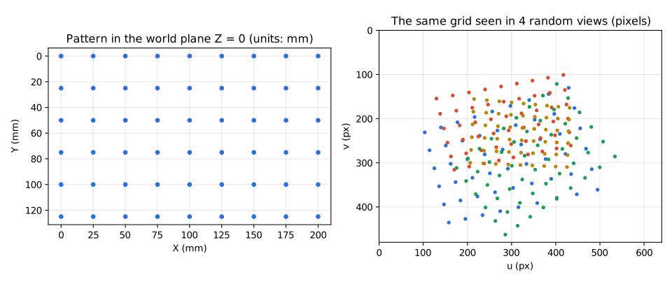
$$s\begin{pmatrix}u\\v\\1\end{pmatrix}=K[\mathbf r_1\ \mathbf r_2\ \mathbf t]\begin{pmatrix}X\\Y\\1\end{pmatrix}\ \Longrightarrow\ H=[\mathbf h_1\ \mathbf h_2\ \mathbf h_3]=\lambda K[\mathbf r_1\ \mathbf r_2\ \mathbf t],$$

with an unknown scalar $\lambda$. $H$ is a 3×3 homography between the pattern plane and the image. It can be estimated from the detected corners with the same normalised DLT used in the previous articles (a homography has 8 degrees of freedom, so 4 correspondences suffice; a 9×6 grid gives 54).

Left: the 9 by 6 grid of pattern points in the plane Z=0. Right: the image of that grid in four random views. — Figure 1. The synthetic setup used below. Left: the 9×6 corner grid with 25 mm squares. Right: four random views of it.

3. Two constraints per view

From $H=\lambda K[\mathbf r_1\ \mathbf r_2\ \mathbf t]$ we get $\mathbf r_1=\lambda^{-1}K^{-1}\mathbf h_1$ and $\mathbf r_2=\lambda^{-1}K^{-1}\mathbf h_2$. Because $R$ is a rotation, $\mathbf r_1$ and $\mathbf r_2$ are orthonormal: $\mathbf r_1^\top\mathbf r_2=0$ and $\|\mathbf r_1\|=\|\mathbf r_2\|$. Substituting gives, for each view,

$$\mathbf h_1^\top B\,\mathbf h_2=0,\qquad \mathbf h_1^\top B\,\mathbf h_1=\mathbf h_2^\top B\,\mathbf h_2,\qquad B=K^{-\top}K^{-1}.$$

$B$ is symmetric, so it is described by the vector $\mathbf b=(B_{11},B_{12},B_{22},B_{13},B_{23},B_{33})^\top$. For $\mathbf h_i=(h_{i1},h_{i2},h_{i3})^\top$ define

$$\mathbf v_{ij}=\big(h_{i1}h_{j1},\ h_{i1}h_{j2}+h_{i2}h_{j1},\ h_{i2}h_{j2},\ h_{i3}h_{j1}+h_{i1}h_{j3},\ h_{i3}h_{j2}+h_{i2}h_{j3},\ h_{i3}h_{j3}\big)^\top,$$

so that $\mathbf h_i^\top B\mathbf h_j=\mathbf v_{ij}^\top\mathbf b$. The two constraints of one view become two linear equations in $\mathbf b$, and $n$ views stack into

$$V\mathbf b=\mathbf 0,\qquad V=\begin{pmatrix}\mathbf v_{12}^\top\\(\mathbf v_{11}-\mathbf v_{22})^\top\\\vdots\end{pmatrix}\in\mathbb R^{2n\times 6}.$$

4. How many views?

$B$ is known only up to scale, so it has 5 degrees of freedom — the same number as the unknowns of $K$. Each view gives 2 equations, so:

$n\ge 3$ views determine $\mathbf b$ (and hence all five intrinsic parameters, including skew) in general.
$n=2$ views are enough if you assume zero skew ($\gamma=0$, i.e. $B_{12}=0$), which adds one more equation. (Zhang also notes that the pattern planes in the different views must not all be parallel to each other, otherwise the constraints are degenerate.)

As in the previous articles, with noisy data we solve $\min_{\|\mathbf b\|=1}\|V\mathbf b\|^2$: $\mathbf b$ is the right singular vector of $V$ for the smallest singular value. The intrinsics then follow from $B$ in closed form (Zhang, Appendix B):

$$v_0=\frac{B_{12}B_{13}-B_{11}B_{23}}{B_{11}B_{22}-B_{12}^2},\quad \lambda'=B_{33}-\frac{B_{13}^2+v_0(B_{12}B_{13}-B_{11}B_{23})}{B_{11}},$$ $$\alpha=\sqrt{\lambda'/B_{11}},\quad \beta=\sqrt{\frac{\lambda' B_{11}}{B_{11}B_{22}-B_{12}^2}},\quad \gamma=-\frac{B_{12}\,\alpha^2\beta}{\lambda'},\quad u_0=\frac{\gamma v_0}{\beta}-\frac{B_{13}\,\alpha^2}{\lambda'}.$$

Notice the square roots. For a real camera $B$ is positive definite, but an estimate from noisy data can fall outside that cone, and then there is no real solution. We will see this actually happen in the experiment. Once $K$ is known, the pose of each view follows from $\mathbf r_1=\lambda K^{-1}\mathbf h_1$, $\mathbf r_2=\lambda K^{-1}\mathbf h_2$, $\mathbf r_3=\mathbf r_1\times\mathbf r_2$, $\mathbf t=\lambda K^{-1}\mathbf h_3$ with $\lambda=1/\|K^{-1}\mathbf h_1\|$ (followed by projection to the nearest rotation matrix).

5. Implementation

The core of the closed-form stage (NumPy). The complete script, including the synthetic data generator, the experiment and both figures, is downloadable.

import numpy as np

def vij(H, i, j):
    h_i, h_j = H[:, i], H[:, j]
    return np.array([h_i[0]*h_j[0], h_i[0]*h_j[1] + h_i[1]*h_j[0], h_i[1]*h_j[1],
                     h_i[2]*h_j[0] + h_i[0]*h_j[2], h_i[2]*h_j[1] + h_i[1]*h_j[2], h_i[2]*h_j[2]])

def calibrate(Hs, N):
    """Hs: list of 3x3 homographies (pattern plane -> pixels).
    N: a similarity that shifts/scales pixel coordinates (conditioning), K = inv(N) @ K_normalised."""
    rows = []
    for H in Hs:
        Hn = N @ H
        rows += [vij(Hn, 0, 1), vij(Hn, 0, 0) - vij(Hn, 1, 1)]
    _, _, Vt = np.linalg.svd(np.array(rows))
    b = Vt[-1] if Vt[-1][0] > 0 else -Vt[-1]
    B11, B12, B22, B13, B23, B33 = b
    den = B11*B22 - B12**2
    v0 = (B12*B13 - B11*B23) / den
    lam = B33 - (B13**2 + v0*(B12*B13 - B11*B23)) / B11
    if den <= 0 or lam/B11 <= 0 or lam*B11/den <= 0:
        raise ValueError("estimated B is not positive definite")
    alpha = np.sqrt(lam / B11)
    beta = np.sqrt(lam * B11 / den)
    gamma = -B12 * alpha**2 * beta / lam
    u0 = gamma * v0 / beta - B13 * alpha**2 / lam
    return np.linalg.inv(N) @ np.array([[alpha, gamma, u0], [0, beta, v0], [0, 0, 1.0]])

The pixel coordinates are shifted to the image centre and divided by 280 (the matrix N) before building $V$, for the same conditioning reason as in the eight-point article; I did not measure its effect separately here.

Sanity checks

With noise-free corners from 5 random views the estimate equals the true $K$ to round-off: $\max|K-K_{\text{true}}|=2.3\times10^{-13}$. With only 2 views and the zero-skew equation the error is $3.2\times10^{-8}$ (still exact for practical purposes, but the system is less well conditioned).

6. Experiment: noise and number of views

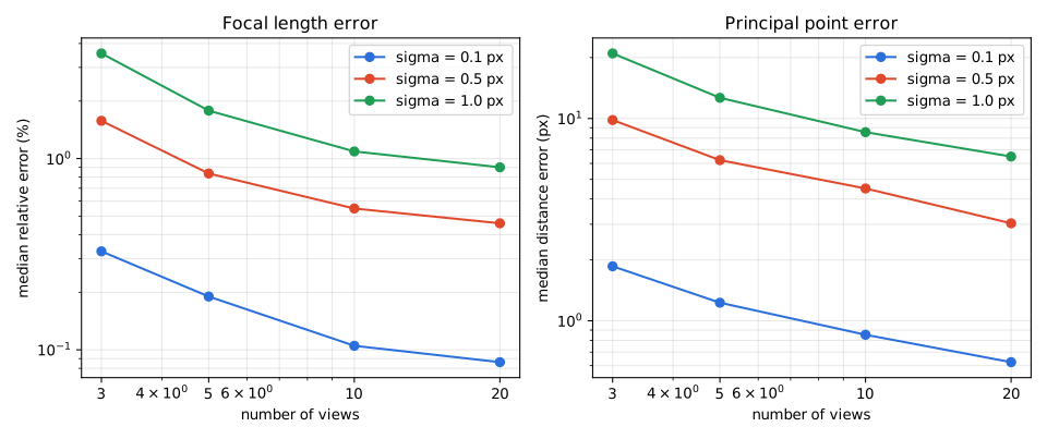
Setup (synthetic, fully reproducible). True intrinsics $\alpha=820$, $\beta=810$, $(u_0,v_0)=(322,238)$, $\gamma=0$, image size 640×480. A 9×6 corner grid with 25 mm squares. Each view has a random pose: rotation angle 15–50° about a random axis, pattern centre 0.45–0.75 m from the camera; poses where any corner leaves the image are rejected. Independent Gaussian noise of standard deviation $\sigma$ is added to every corner, a homography is estimated per view, and $K$ is computed with the closed form with skew free. For each of the 12 combinations of $\sigma\in\{0.1,0.5,1.0\}$ px and $n\in\{3,5,10,20\}$ views I ran 300 trials (NumPy seed 2026) and report the median over the successful trials of: the mean relative error of $\alpha$ and $\beta$ (%), and the distance between estimated and true principal point (px). No lens distortion is simulated and no non-linear refinement is applied.

σ (px)	3 views	5 views	10 views	20 views
0.1	0.327 % / 1.86 px	0.190 % / 1.23 px	0.105 % / 0.85 px	0.086 % / 0.62 px
0.5	1.576 % / 9.83 px	0.836 % / 6.22 px	0.548 % / 4.51 px	0.459 % / 3.03 px
1.0	3.550 % / 20.98 px ^*	1.782 % / 12.66 px	1.090 % / 8.56 px	0.901 % / 6.48 px

Each cell: median focal-length error / median principal-point error. ^* In 0.7 % of the 300 trials (3 views, σ=1 px) the estimated $B$ was not positive definite and the closed form failed; all other cells had 0 % failures, and the medians exclude failed trials.

Log-log plots of median focal-length error and principal-point error against the number of views for three noise levels — Figure 2. Median focal-length error (left) and principal-point error (right) versus the number of views, one curve per noise level. Output of the script in this article.

What the numbers say

Error scales roughly with the noise. With 10 views the focal error is 0.105 %, 0.548 % and 1.090 % for $\sigma=0.1,0.5,1.0$ px — ratios of about 5.2× and 2.0× for noise ratios of 5× and 2×.
More views help, with diminishing returns. At $\sigma=0.5$ px going from 3 to 5 views cuts the focal error from 1.58 % to 0.84 % (−47 %), whereas going from 10 to 20 views cuts it only from 0.55 % to 0.46 % (−16 %).
The principal point is the harder parameter. At 10 views and $\sigma=0.5$ px its median error is 4.5 px, which is of the same size as the focal error expressed in pixels (0.548 % of about 815 px ≈ 4.5 px); a 0.5 px corner noise therefore becomes a several-pixel uncertainty in where the optical axis hits the sensor.
The minimum number of views is fragile. With 3 views and 1 px noise the error is 3.6 % and the closed form occasionally fails altogether.
Single runs vary. One illustrative run ($\sigma=0.5$ px, 10 views, seed 3) gave $\alpha=810.2$, $\beta=802.0$, $(u_0,v_0)=(325.6,241.2)$, skew $-0.62$: errors of 1.2 % and 1.0 % on the focal lengths, roughly twice the median. A practical calibration should not rely on one lucky or unlucky set of photos.

Limitations. The data are synthetic, noise is isotropic Gaussian with the same $\sigma$ for all corners, there is no lens distortion and no outlier corner, the pose distribution is one particular choice, and I only evaluated the closed-form stage. Real calibrations add the radial-distortion estimate and a non-linear refinement that minimises the reprojection error of all corners over all parameters, which Zhang reports as part of the procedure; I did not quantify how much it improves on the closed form here. Results on real cameras also depend on the quality of the corner detector.

7. Practical takeaways

Use at least 5 views, and ideally 10 or more, with the pattern tilted by different amounts and in different directions — not 3 nearly parallel ones.
Keep the pattern large in the image and spread it over the whole field of view; noise in corner positions maps directly into error in $K$.
Treat the closed form as an initialisation. For real work refine all parameters (and distortion) by minimising reprojection error, and check the final RMS reprojection error and the spread between independent calibrations.
If $B$ is not positive definite, the data are inconsistent with the model (too few or too similar views, a corner detection error): collect more views instead of forcing a solution.
With $K$ known you can undistort the images, estimate the essential matrix instead of $F$ as in the eight-point article, and triangulate in metric units as in the triangulation article.

Need 3D reconstruction, a chatbot agent or a custom AI tool?
I build these as a freelancer. Describe your project in a few sentences and I will reply with questions and a fixed-scope quote.

Ask for a quote 3D reconstruction service

References

Z. Zhang. “A flexible new technique for camera calibration.” IEEE Transactions on Pattern Analysis and Machine Intelligence 22(11):1330–1334, November 2000. doi:10.1109/34.888718. (Also Microsoft Research technical report MSR-TR-98-71, publication page.)
R. Hartley and A. Zisserman. Multiple View Geometry in Computer Vision, 2nd ed. Cambridge University Press, 2004. ISBN 978-0-521-54051-3. Publisher page.

Code: zhang_calibration.py (Python 3.12, NumPy, Matplotlib). All numbers in Sections 5–6 are the output of this script.