Triangulation: from two views to a 3D point
1. Context
Every 3D reconstruction pipeline built from images — structure from motion, photogrammetry, stereo — eventually asks the same question: given where a point appears in two or more images, and given the cameras, where is it in 3D? Answering it is called triangulation. It is the “recover the point” step once the cameras are known (or estimated).
In a perfect world the answer is just the intersection of two rays. In real images, pixel coordinates are noisy, the two rays are skew and almost never meet, and we need a principled way to pick the best point. This article derives the standard linear solution, implements it, and tests how it behaves.
2. The pinhole camera
A 3D point in homogeneous coordinates \(\mathbf{X}=(X,Y,Z,1)^\top\) is projected to the image point \(\mathbf{x}=(u,v,1)^\top\) by a \(3\times4\) camera matrix \(P\):
$$\lambda\,\mathbf{x} = P\,\mathbf{X},\qquad P = K\,[\,R \mid \mathbf{t}\,],\qquad K=\begin{bmatrix} f_x & 0 & c_x\\ 0 & f_y & c_y\\ 0&0&1\end{bmatrix}$$Here \(K\) holds the intrinsics (focal lengths \(f_x,f_y\) in pixels and principal point \((c_x,c_y)\)), and \([R\mid\mathbf t]\) are the extrinsics: the rotation and translation from world to camera coordinates. The scalar \(\lambda\) is the unknown projective depth. The symbol \(\simeq\) is often used for “equal up to scale”.
3. Why the rays do not meet
Each observed pixel defines a ray from the camera centre. With exact data the two rays intersect at the true point \(\mathbf X\). With noisy pixels, the rays in 3D are generally skew — they pass each other without touching. The top-down view below is a 2D slice, where two lines always cross, so it only shows the other half of the story: noise moves the crossing point away from the truth, mostly along the viewing direction (depth).
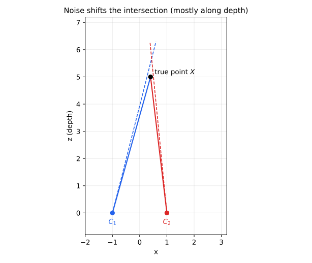
We therefore need a criterion for the “best” point. Two natural choices are (a) an algebraic criterion that leads to a linear system, and (b) the geometric reprojection error.
4. Linear triangulation (DLT)
The relation \(\lambda\mathbf x=P\mathbf X\) says \(\mathbf x\) and \(P\mathbf X\) are parallel, so their cross product vanishes:
$$\mathbf{x}\times(P\mathbf{X})=\mathbf 0 .$$Let \(\mathbf p_i^\top\) be the \(i\)-th row of \(P\) and \(\mathbf x=(u,v,1)^\top\). Expanding the cross product gives three equations, only two of which are linearly independent:
$$u\,\mathbf p_3^\top\mathbf X-\mathbf p_1^\top\mathbf X=0,\qquad v\,\mathbf p_3^\top\mathbf X-\mathbf p_2^\top\mathbf X=0 .$$With two views \((P,\mathbf x=(u,v,1)^\top)\) and \((P',\mathbf x'=(u',v',1)^\top)\) we stack four equations into \(A\mathbf X=\mathbf 0\):
$$A=\begin{bmatrix} u\,\mathbf p_3^\top-\mathbf p_1^\top\\ v\,\mathbf p_3^\top-\mathbf p_2^\top\\ u'\,\mathbf p_3'^\top-\mathbf p_1'^\top\\ v'\,\mathbf p_3'^\top-\mathbf p_2'^\top\end{bmatrix}\in\mathbb R^{4\times4} .$$Because \(\mathbf X\) is homogeneous we only know it up to scale, so we solve
$$\hat{\mathbf X}=\arg\min_{\|\mathbf X\|=1}\ \|A\mathbf X\|^2 ,$$whose solution is the right singular vector of \(A\) associated with the smallest singular value. If \(A=U\Sigma V^\top\), then \(\hat{\mathbf X}\) is the last column of \(V\). Finally we dehomogenise: \((X,Y,Z)=(\hat X_1,\hat X_2,\hat X_3)/\hat X_4\).
5. Implementation
Below is the core of the implementation (NumPy). The complete script, including the experiment and the figures in this article, is downloadable.
import numpy as np

def triangulate_dlt(P1, P2, x1, x2):
    """Homogeneous linear triangulation: solve A X = 0 by SVD."""
    A = np.vstack([
        x1[0] * P1[2] - P1[0],
        x1[1] * P1[2] - P1[1],
        x2[0] * P2[2] - P2[0],
        x2[1] * P2[2] - P2[1],
    ])
    _, _, Vt = np.linalg.svd(A)
    X = Vt[-1]              # right singular vector of the smallest singular value
    return X[:3] / X[3]     # dehomogenise
For comparison I also implemented the midpoint method: back-project both pixels to rays \(\mathbf c_i+s_i\mathbf d_i\), find \((s_1,s_2)\) minimising the distance between the rays, and return the midpoint of that shortest segment.
Sanity check
Before trusting any numbers, I triangulated a point from noise-free projections. The reconstruction error was 1.13e-15 (floating-point round-off), as it must be when the rays intersect exactly.
6. Experiment: how does baseline affect accuracy?
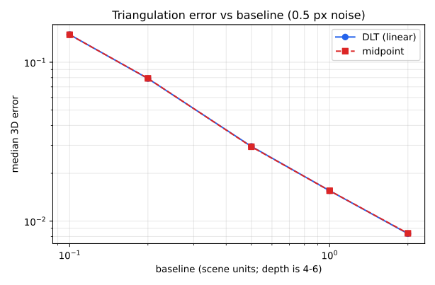
Setup (synthetic, fully reproducible). Intrinsics \(f_x=f_y=800\) px, principal point \((320,240)\). Two cameras placed symmetrically on the x-axis at \(\pm b/2\), both looking at \((0,0,5)\). Random 3D points with \(x,y\in[-1,1]\), \(z\in[4,6]\). Each projection receives independent Gaussian noise with \(\sigma=0.5\) px. For each baseline \(b\) I triangulate 2000 points (NumPy random seed 7) and report the median Euclidean 3D error, in the same units as the scene.
| Baseline b | DLT median error | Midpoint median error |
|---|---|---|
| 0.10 | 0.1492 | 0.1489 |
| 0.20 | 0.0789 | 0.0792 |
| 0.50 | 0.0295 | 0.0294 |
| 1.00 | 0.0155 | 0.0155 |
| 2.00 | 0.0083 | 0.0084 |
What the numbers say
- Baseline dominates accuracy. Increasing the baseline 20× (0.1 → 2.0) reduced the median error by about 18× (0.149 → 0.0083), i.e. roughly inversely proportional to the baseline in this regime.
- This matches the rectified-stereo intuition. For two parallel cameras with focal length \(f\) and baseline \(B\), depth is \(Z=fB/d\) where \(d\) is the disparity. Differentiating, a disparity error \(\delta d\) produces a depth error \(\delta Z\approx \dfrac{Z^2}{fB}\,\delta d\): depth error grows with the square of the distance and shrinks with the baseline.
- In this setup DLT and midpoint are practically identical. The two methods differ by less than 1% at every baseline. This experiment (small noise, well-conditioned geometry, both cameras looking at the scene centre) is simply not one that separates them. I make no claim about other regimes; for a systematic comparison of methods see Hartley & Sturm (1997).
Limitations. The data are synthetic, noise is Gaussian and isotropic, camera calibration is assumed exact, and I did not compare against the optimal (minimum reprojection error) method. Real pipelines add lens distortion, outlier matches and calibration error — each of which needs its own treatment (robust estimation, bundle adjustment).
7. Practical takeaways
- Use as large a baseline as the matching algorithm tolerates: it directly reduces depth uncertainty.
- Check your code with noise-free data first; it should reproduce the point to round-off.
- Treat DLT as a fast, solid initial estimate; refine by minimising reprojection error when accuracy matters.
- Always report the metric you actually care about (reprojection error, 3D error) — they are not the same as the algebraic residual.
I build these as a freelancer. Describe your project in a few sentences and I will reply with questions and a fixed-scope quote.
Ask for a quote See services
References
- R. Hartley and A. Zisserman. Multiple View Geometry in Computer Vision, 2nd ed. Cambridge University Press, 2004. ISBN 978-0-521-54051-3. (Chapter 12, “Structure computation”.) Publisher page.
- R. I. Hartley and P. Sturm. “Triangulation.” Computer Vision and Image Understanding 68(2):146–157, November 1997. doi:10.1006/cviu.1997.0547.