The eight-point algorithm and why normalisation matters
1. Context
In the previous article we assumed the two cameras were known and recovered a 3D point from its two images. In practice the cameras are rarely given. What you have is a set of matches: pixel pairs that look like the same physical point in two photos. The first step of most structure-from-motion pipelines is to extract from these matches a single 3×3 matrix, the fundamental matrix \(F\), that encodes the relative geometry of the two views.
The classic way to compute it from eight or more matches is the eight-point algorithm. Longuet-Higgins (1981) introduced the algorithm for calibrated cameras; for a long time afterwards it was considered too sensitive to noise to be useful. Hartley (1997) showed that a very simple preprocessing step — translating and scaling the pixel coordinates — makes the same linear algorithm competitive with iterative methods. This article derives the algorithm, implements both versions, and measures the difference.
2. Epipolar geometry and the fundamental matrix
Take a 3D point \(\mathbf X\) seen by two cameras at image points \(\mathbf x=(u,v,1)^\top\) and \(\mathbf x'=(u',v',1)^\top\). The two camera centres \(C,C'\) and \(\mathbf X\) span a plane, the epipolar plane. Both image points lie on its intersection with each image plane, so \(\mathbf x'\) must lie on a line in the second image that depends only on \(\mathbf x\) and the camera geometry. The line joining \(C\) and \(C'\) (the baseline) pierces the image planes at the epipoles \(\mathbf e,\mathbf e'\).
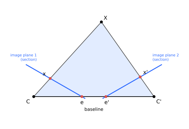
This geometric fact is expressed algebraically by the epipolar constraint
$$\mathbf x'^\top F\,\mathbf x = 0 ,$$where, for cameras \(P=K[I\mid\mathbf 0]\) and \(P'=K'[R\mid\mathbf t]\), the fundamental matrix is \(F=K'^{-\top}[\mathbf t]_\times R\,K^{-1}\), with \([\mathbf t]_\times\) the skew-symmetric matrix of the cross product (Hartley & Zisserman, Ch. 9). Two properties matter for estimation: \(F\) is defined only up to scale, and it has rank 2 (because \([\mathbf t]_\times\) does), leaving 7 degrees of freedom. If the cameras are calibrated, \(E=K'^\top F K\) is the essential matrix that Longuet-Higgins worked with.
3. The linear algorithm
Write out \(\mathbf x'^\top F\mathbf x=0\) for one match. With \(F=(f_{ij})\), multiplying out gives
$$u'u\,f_{11}+u'v\,f_{12}+u'\,f_{13}+v'u\,f_{21}+v'v\,f_{22}+v'\,f_{23}+u\,f_{31}+v\,f_{32}+f_{33}=0 ,$$which is linear in the nine unknowns \(\mathbf f=(f_{11},\dots,f_{33})^\top\). Each match therefore contributes one row \((u'u,\;u'v,\;u',\;v'u,\;v'v,\;v',\;u,\;v,\;1)\), and stacking \(N\ge 8\) matches gives
$$A\,\mathbf f=\mathbf 0,\qquad A\in\mathbb R^{N\times 9}.$$With eight exact matches in general position \(A\) has rank 8 and the solution is its null vector. With noisy data and \(N\ge 8\) we instead solve
$$\hat{\mathbf f}=\arg\min_{\|\mathbf f\|=1}\ \|A\mathbf f\|^2 ,$$whose solution is the right singular vector of \(A\) for the smallest singular value, exactly as in the triangulation article. The reshaped matrix \(\hat F\) will in general have rank 3, which violates the epipolar geometry (the epipolar lines would not all meet at one point). We therefore replace it by the closest rank-2 matrix in the Frobenius norm: if \(\hat F=U\,\mathrm{diag}(\sigma_1,\sigma_2,\sigma_3)\,V^\top\), set
$$F=U\,\mathrm{diag}(\sigma_1,\sigma_2,0)\,V^\top .$$4. Why raw pixel coordinates hurt: conditioning
Look at the entries of one row of \(A\). With pixel coordinates of order hundreds, \(u'u\) is of order \(10^5\), terms like \(u\) or \(u'\) are of order \(10^2\), and the last entry is \(1\). The columns of \(A\) differ in scale by up to five orders of magnitude. The SVD minimises \(\|A\mathbf f\|\) in the Euclidean sense, so it effectively gives the large columns far more weight than the small ones; the problem is badly conditioned.
Hartley normalisation fixes the scale before building \(A\). For each image separately, find a similarity transform \(T\) that moves the centroid of the points to the origin and scales them so that their mean distance from the origin is \(\sqrt 2\):
$$\tilde{\mathbf x}_i=T\mathbf x_i,\qquad \tilde{\mathbf x}'_i=T'\mathbf x'_i .$$Run the algorithm above on the normalised points to get \(\tilde F\), then undo the normalisation. Since \(\tilde{\mathbf x}'^\top\tilde F\tilde{\mathbf x}=\mathbf x'^\top (T'^\top\tilde F\,T)\,\mathbf x\), the answer in pixel coordinates is
$$F=T'^\top\,\tilde F\,T .$$(Hartley & Zisserman describe this as the normalized 8-point algorithm, Ch. 11.)
5. Implementation
The core of the implementation (NumPy). The complete script, including the experiment and both figures, is downloadable.
import numpy as np

def normalise(pts):
    """Hartley normalisation: centroid -> origin, mean distance -> sqrt(2)."""
    c = pts.mean(axis=0)
    d = np.sqrt(((pts - c) ** 2).sum(axis=1)).mean()
    s = np.sqrt(2) / d
    T = np.array([[s, 0, -s * c[0]], [0, s, -s * c[1]], [0, 0, 1.0]])
    return np.column_stack([pts, np.ones(len(pts))]) @ T.T, T

def eight_point(p1, p2, normalised):
    """p1, p2: (N,2) pixel coordinates, N>=8. Convention: x2^T F x1 = 0."""
    if normalised:
        h1, T1 = normalise(p1); h2, T2 = normalise(p2)
    else:
        h1 = np.column_stack([p1, np.ones(len(p1))])
        h2 = np.column_stack([p2, np.ones(len(p2))])
        T1 = T2 = np.eye(3)
    A = np.stack([np.kron(b, a) for a, b in zip(h1, h2)])   # N x 9
    _, S, Vt = np.linalg.svd(A)
    F = Vt[-1].reshape(3, 3)
    U, D, Vt2 = np.linalg.svd(F)                             # enforce rank 2
    F = U @ np.diag([D[0], D[1], 0.0]) @ Vt2
    F = T2.T @ F @ T1                                        # denormalise
    return F / np.linalg.norm(F), S
Sanity check
I generated 20 noise-free matches from a known \(F_{\text{true}}\). Both variants recover it to round-off: \(\|F-F_{\text{true}}\|=4.7\times10^{-15}\) (raw) and \(5.9\times10^{-15}\) (normalised), after fixing the sign. Without noise the two algorithms are therefore equally correct; any difference must come from numerics.
6. Experiment: raw vs. normalised
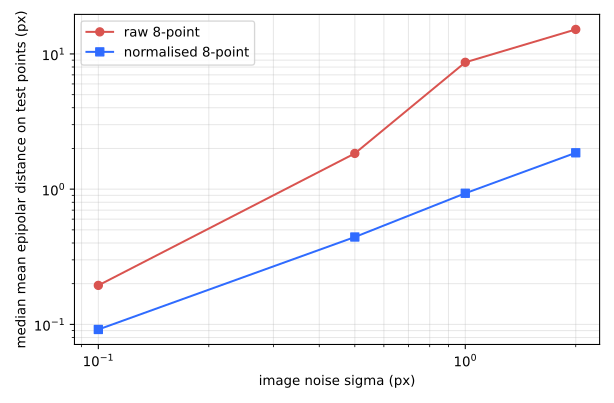
Setup (synthetic, fully reproducible). Intrinsics \(f=800\) px, principal point \((320,240)\), identical for both cameras. Camera 1 is \([I\mid\mathbf 0]\); camera 2 is rotated by \(-8^\circ\) about the y-axis with \(\mathbf t=(-1,\,0.05,\,0.05)\). Random 3D points with \(x\in[-1,1]\), \(y\in[-0.75,0.75]\), \(z\in[4,8]\). Each trial uses \(N=20\) matches with independent Gaussian noise of standard deviation \(\sigma\) added to every pixel coordinate. The estimated \(F\) is scored on 1000 separate noise-free matches that were not used for estimation, using the mean symmetric point-to-epipolar-line distance in pixels. I report the median over 300 trials (NumPy seed 11).
Conditioning. For noise-free data, the median ratio of the largest to the eighth singular value of \(A\) is \(4.6\times10^{5}\) for raw pixel coordinates and \(18.0\) after normalisation (seed 5, 300 trials).
| Noise σ (px) | Raw 8-point (px) | Normalised 8-point (px) |
|---|---|---|
| 0.00 | 0.0000 | 0.0000 |
| 0.10 | 0.1943 | 0.0917 |
| 0.50 | 1.8377 | 0.4428 |
| 1.00 | 8.6689 | 0.9326 |
| 2.00 | 15.1767 | 1.8583 |
What the numbers say
- Normalisation shrinks the condition number by four orders of magnitude (about \(4.6\times10^{5}\) to 18) in this setup, which is the numerical reason the two variants behave differently once noise is present.
- The normalised estimate degrades gracefully. Its held-out error is close to the injected noise level and grows roughly in proportion to \(\sigma\): 0.092, 0.443, 0.933 and 1.858 px for \(\sigma=0.1, 0.5, 1, 2\) px.
- The raw estimate is far worse and grows faster than the noise. At \(\sigma=1\) px its error is 8.67 px versus 0.93 px (9.3× larger); at \(\sigma=0.5\) it is 4.2× larger and at \(\sigma=0.1\) it is 2.1× larger.
- Without noise there is no difference, as the sanity check showed: normalisation is about numerical stability, not about a different solution.
Limitations. The data are synthetic, noise is Gaussian and isotropic, there are no outlier matches, I used a single fixed camera geometry with \(N=20\) matches, and I measured only epipolar distance on held-out points. I did not compare against iterative (maximum-likelihood) estimators; Hartley (1997) reports such comparisons on real images and finds the normalised algorithm comparable with the best iterative methods. Real matches also contain outliers, which require robust estimation (RANSAC) around the eight-point solver.
7. Practical takeaways
- Always normalise the coordinates before running a linear (DLT-style) estimator; it costs a few lines and removes a major source of numerical error.
- Enforce rank 2 after the SVD, and denormalise at the end.
- Test with noise-free synthetic data first, then evaluate on held-out points, not on the points you fitted.
- Use the eight-point result as an initial estimate; with real data, wrap it in RANSAC and refine by minimising a geometric error.
- Once \(F\) (or \(E\)) is known and the cameras are recovered, you can triangulate the points as in the previous article.
I build these as a freelancer. Describe your project in a few sentences and I will reply with questions and a fixed-scope quote.
Ask for a quote See services
References
- H. C. Longuet-Higgins. “A computer algorithm for reconstructing a scene from two projections.” Nature 293:133–135, 10 September 1981. doi:10.1038/293133a0.
- R. I. Hartley. “In defense of the eight-point algorithm.” IEEE Transactions on Pattern Analysis and Machine Intelligence 19(6):580–593, June 1997. doi:10.1109/34.601246.
- R. Hartley and A. Zisserman. Multiple View Geometry in Computer Vision, 2nd ed. Cambridge University Press, 2004. ISBN 978-0-521-54051-3. (Chapter 9, epipolar geometry and the fundamental matrix; Chapter 11, computation of the fundamental matrix.) Publisher page.