PCA through the SVD: derivation, numerical stability and compressing sensor data
1. Background
An IoT node that reads several correlated sensors (temperature, humidity, vibration at several positions) usually has fewer real sources of variation than channels. A few scores can then be sent instead of the whole measurement vector, and the part of the data that those scores cannot explain can be used to spot a faulty sensor. Principal component analysis (PCA) is the standard tool for both: Pearson (1901) studied the lines and planes of closest fit to a cloud of points, Hotelling (1933) named the method and derived it through variances, and Jolliffe and Cadima (2016) review the variants. This post derives PCA from the SVD, checks the identities numerically, compares two ways of computing it for stability, and measures the result on a simulated sensor array.
2. Derivation
Let \(X\in\mathbb{R}^{n\times d}\) hold \(n\) samples of \(d\) channels, \(\mu\) the column mean and \(X_c=X-\mathbf 1\mu^\top\) the centred matrix. The sample covariance is \(S=X_c^\top X_c/(n-1)\). The unit direction \(v\) that maximises the variance of the projection solves
$$\max_{\|v\|=1}\ \operatorname{Var}(X_c v)=\max_{\|v\|=1}\ v^\top S v,$$and it is the eigenvector of \(S\) with the largest eigenvalue (a Lagrange multiplier gives \(Sv=\lambda v\), and the variance attained is \(\lambda\)). The second direction is found the same way in the orthogonal complement, and so on. Write the thin SVD of \(X_c\):
$$X_c=U\Sigma V^\top,\qquad U^\top U=V^\top V=I,\quad \Sigma=\operatorname{diag}(\sigma_1\ge\sigma_2\ge\dots\ge0).$$Substituting into \(S\) gives \(S=V\,\dfrac{\Sigma^2}{n-1}\,V^\top\). The principal axes are therefore the columns of \(V\), their variances are
$$\lambda_i=\frac{\sigma_i^2}{n-1},$$and the scores (coordinates along the axes) are \(T=X_cV=U\Sigma\). Keeping \(k\) components gives the rank-\(k\) approximation \(\hat X_k=X_cV_kV_k^\top\). The Eckart–Young theorem (1936) states that \(\hat X_k\) is the matrix of rank at most \(k\) closest to \(X_c\) in the Frobenius norm, and
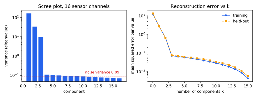
$$\|X_c-\hat X_k\|_F^2=\sum_{i>k}\sigma_i^2,\qquad \text{explained variance ratio}=\frac{\sum_{i\le k}\sigma_i^2}{\sum_i\sigma_i^2}.$$The reconstruction error can therefore be read off the singular spectrum: the scree plot shows both how many components to keep and what is lost.
Residuals and fault detection. For a new sample \(x\), the residual is \(r=(I-V_kV_k^\top)(x-\mu)\) and \(Q=\|r\|^2\) (the Q statistic, also called SPE). Jackson and Mudholkar (1979) study the use of this statistic for process control: if the \(k\)-component model still holds, \(Q\) is small, while a sensor that departs from the usual correlation structure inflates \(Q\). If the fault is an offset \(\delta\) added to channel \(c\), the squared norm of the residual due to the offset alone is
$$\delta^2\Bigl(1-\sum_{j\le k}V_{cj}^2\Bigr),$$so a channel with large loadings on the principal components (\(\sum_{j\le k}V_{cj}^2\) close to 1) “hides” part of the offset inside the subspace and is harder to detect.
3. Two ways to compute it, and numerical stability
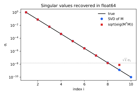
Route 1: the SVD of \(X_c\). Route 2: form \(S=X_c^\top X_c/(n-1)\) and solve a symmetric eigenproblem. They are algebraically identical, but forming \(X_c^\top X_c\) squares the condition number: \(\kappa(X_c^\top X_c)=\kappa(X_c)^2\). A symmetric eigensolver returns eigenvalues with absolute error of order \(\varepsilon\,\|S\|\) (\(\varepsilon\approx2.2\cdot10^{-16}\) in float64), so singular values \(\sigma_i=\sqrt{\lambda_i}\) below about \(\sqrt{\varepsilon}\,\sigma_1\approx1.5\cdot10^{-8}\sigma_1\) lose all significant digits; the SVD applied directly keeps an absolute error of order \(\varepsilon\,\sigma_1\) (Golub and Van Loan, 2013). This is the same squaring of \(\kappa\) that slows gradient descent in the post on gradient descent and the condition number.
4. Implementation
The full script (data generation, four experiments, two figures; about 2 seconds) is available for download. The core:
def pca_svd(X, k):
    """PCA of the rows of X via thin SVD of the centred matrix."""
    mu = X.mean(0)
    _, s, Vt = np.linalg.svd(X - mu, full_matrices=False)
    return mu, Vt[:k], s                         # lambda_i = s_i**2 / (n - 1)

def pca_cov(X, k):
    """PCA via eigendecomposition of the sample covariance (forms X^T X)."""
    mu = X.mean(0)
    Xc = X - mu
    w, V = np.linalg.eigh(Xc.T @ Xc / (len(X) - 1))
    order = np.argsort(w)[::-1]
    return mu, V[:, order[:k]].T, w[order]

def reconstruct(X, mu, comps):
    return (X - mu) @ comps.T @ comps + mu

# Q statistic (SPE) of each row, threshold = 99th percentile of the training Q
spe = lambda X: np.sum((X - reconstruct(X, mu, comps)) ** 2, 1)
5. Experimental setup
Data (synthetic, fully reproducible). \(d=16\) sensor channels driven by \(k=3\) independent Gaussian latent sources with standard deviations 3, 2 and 1. The loading matrix \(A\in\mathbb{R}^{16\times3}\) is standard Gaussian, each channel has its own offset (standard deviation 2) and independent Gaussian noise of standard deviation 0.3: \(x=Az+\text{offset}+\text{noise}\). Each seed (0–19) draws a new loading matrix, 1,000 training samples and 1,000 new test samples. The model is fitted on the training set; every error reported in Section 7 is computed on the test set.
6. Sanity checks (seed 0)
- The two routes agree on well-conditioned data. \(\max_i|\sigma_i^2/(n-1)-\lambda_i|=8.5\cdot10^{-14}\) over all 16 values and, after fixing signs, the first 3 component vectors differ by at most \(8.6\cdot10^{-16}\). The leading covariance eigenvalues are 161.3, 33.41, 9.502, then 0.1092, 0.1062, 0.09915: the first three components carry 99.44 % of the total variance and the rest lie close to the noise variance \(0.3^2=0.09\).
- The Eckart–Young identity. \(\|X_c-\hat X_k\|_F^2\) and \(\sum_{i>k}\sigma_i^2\) agree to every printed digit:
\(k\) \(\|X_c-\hat X_k\|_F^2\) \(\sum_{i>k}\sigma_i^2\) 1 44,014.109772 44,014.109772 2 10,635.719080 10,635.719080 3 1,143.290310 1,143.290310 5 928.087154 928.087154 8 639.974303 639.974303
7. Experiment 1: compression and fault detection on held-out data
| Quantity (\(k=3\), mean ± standard deviation over 20 seeds) | Result |
|---|---|
| Held-out reconstruction RMSE per value | 0.2708 ± 0.0015 (noise-only expectation: \(0.3\sqrt{13/16}=0.2704\)) |
| Storage | 16 floats become 3 scores per sample (5.33× smaller), plus a 3×16 basis stored once |
| False-alarm rate on normal held-out data (threshold = 99th percentile of training Q) | 1.27 % ± 0.37 % (target 1 %) |
With \(k\) equal to the true number of sources, what remains in the residual is almost pure noise: the noise has \(d\) independent components, the projection keeps \(k\) of them, so the residual holds on average \(\sigma_n^2(d-k)/d\) per value, an RMSE of \(0.3\sqrt{13/16}=0.2704\), close to the measured 0.2708. The false-alarm rate of 1.27 % is slightly above the 1 % target, consistent with the threshold being estimated from the residuals of the same set used to fit the model.
Detecting a one-channel offset fault. On the test set, an offset \(\delta\) is added to one channel (each of the 16 channels is tried in turn) and the fraction of samples whose \(Q\) exceeds the threshold is recorded:
| Offset \(\delta\) (relative to noise std 0.3) | Detection rate, mean over 16 channels | Hardest channel (mean over 20 seeds) |
|---|---|---|
| 0.5 (1.7×) | 4.0 % ± 0.6 | 2.5 % |
| 1.0 (3.3×) | 23.9 % ± 2.1 | 11.6 % |
| 2.0 (6.7×) | 94.8 % ± 1.0 | 74.2 % |
| 3.0 (10×) | 99.9 % ± 0.2 | 98.7 % |
- Small faults are almost invisible: an offset of 1.7 noise standard deviations is detected in only 4 % of samples; from about 7 times upward the mean rate exceeds 94 %.
- Channels differ. At \(\delta=2\), the hardest channel reaches only 74.2 % against a 94.8 % average, in the direction of the formula \(\delta^2(1-\sum_{j\le k}V_{cj}^2)\) in Section 2: the part of the offset that falls in the principal subspace leaves no residual.
8. Experiment 2: when the covariance route breaks
Build \(M=U\operatorname{diag}(\sigma)V^\top\) of size 200×10 with random orthogonal \(U,V\) and \(\sigma\) log-spaced from 1 down to \(10^{-10}\) (\(\kappa(M)=10^{10}\), \(\kappa(M^\top M)=10^{20}\)), then recover \(\sigma\) both ways:
| \(i\) | true \(\sigma_i\) | Relative error, SVD of \(M\) | Relative error, \(\sqrt{\text{eig}(M^\top M)}\) |
|---|---|---|---|
| 1 | 1.000e+00 | 1.1e-16 | 1.1e-16 |
| 2 | 7.743e-02 | 1.8e-16 | 2.5e-15 |
| 3 | 5.995e-03 | 4.3e-16 | 6.1e-13 |
| 4 | 4.642e-04 | 8.2e-16 | 8.9e-12 |
| 5 | 3.594e-05 | 1.4e-13 | 5.3e-09 |
| 6 | 2.783e-06 | 1.9e-12 | 1.5e-06 |
| 7 | 2.154e-07 | 5.7e-12 | 9.1e-05 |
| 8 | 1.668e-08 | 2.2e-10 | 1.1e-01 |
| 9 | 1.292e-09 | 1.3e-09 | 4.9e+00 |
| 10 | 1.000e-10 | 9.4e-09 | 1.0e+00 (computed eigenvalue is −2.93e-17, clipped to 0) |
- The SVD keeps the absolute error below \(\varepsilon\sigma_1\). The relative error grows as \(\sigma_i\) shrinks but the absolute error stays tiny (of order \(10^{-18}\) at \(i=8\) and \(9\)), consistent with \(\varepsilon\sigma_1=2.2\cdot10^{-16}\) as a bound.
- The covariance route loses accuracy from \(i=6\) (relative error \(1.5\cdot10^{-6}\)) and fails outright from \(i=8\): \(\sigma_8=1.7\cdot10^{-8}\) sits at the threshold \(\sqrt{\varepsilon}\sigma_1=1.5\cdot10^{-8}\) with an 11 % error; \(\sigma_9\) is off by nearly a factor of 6; \(\sigma_{10}^2=10^{-20}\) lies below the numerical noise \(\varepsilon\sigma_1^2=2.2\cdot10^{-16}\), so the computed eigenvalue is negative.
Limitations. The data are synthetic and Gaussian, with exactly 3 latent sources and independent noise of equal size; real sensors have non-Gaussian noise, drift and distributions that change with conditions. \(k=3\) is known in advance; in practice \(k\) must be chosen from the scree plot or by cross-validation. The Q threshold is the empirical percentile of the training set, not the analytic approximation of Jackson and Mudholkar, and the training set is assumed free of faults. Only one fault type was tried (a constant offset on one channel), not stuck sensors, slow drift or several failing channels at once. PCA is linear; nonlinear relations between channels need other methods. The stability experiment uses a purpose-built matrix with \(\kappa=10^{10}\), far more extreme than the sensor data of Section 6 (the ratio of largest to smallest singular value is only about 40, so the two routes agree). No run time or energy was measured on an embedded device.
9. Practical conclusions
- Compute PCA by the SVD of the centred matrix; the axes are the columns of \(V\), the variances are \(\sigma_i^2/(n-1)\), the scores are \(U\Sigma\).
- Read the reconstruction error off the singular spectrum: \(\sum_{i>k}\sigma_i^2\) is the minimum squared error over all rank-\(k\) approximations.
- The covariance route is fine when the singular values of interest exceed about \(10^{-8}\sigma_1\); below that, use the SVD.
- Once a \(k\)-component model exists, the Q statistic of the residual is a cheap sensor-fault detector: here 1.3 % false alarms and over 94 % detection of an offset of 6.7 noise standard deviations, but only 4 % for 1.7.
- Check channel by channel: a channel with large loadings on the principal components is considerably harder to monitor.
I take projects as a freelancer. Describe yours in a few sentences and I will reply with questions and a fixed-scope quote.
Get a quote See services
References
- K. Pearson. “On lines and planes of closest fit to systems of points in space.” The London, Edinburgh, and Dublin Philosophical Magazine and Journal of Science, series 6, vol. 2, no. 11, 1901, pp. 559–572. doi:10.1080/14786440109462720.
- H. Hotelling. “Analysis of a complex of statistical variables into principal components.” Journal of Educational Psychology 24(6), 1933, pp. 417–441. doi:10.1037/h0071325.
- C. Eckart and G. Young. “The approximation of one matrix by another of lower rank.” Psychometrika 1(3), 1936, pp. 211–218. doi:10.1007/BF02288367.
- J. E. Jackson and G. S. Mudholkar. “Control procedures for residuals associated with principal component analysis.” Technometrics 21(3), 1979, pp. 341–349. doi:10.1080/00401706.1979.10489779.
- I. T. Jolliffe and J. Cadima. “Principal component analysis: a review and recent developments.” Philosophical Transactions of the Royal Society A 374(2065), 20150202, 2016. doi:10.1098/rsta.2015.0202.
- G. H. Golub and C. F. Van Loan. Matrix Computations, 4th edition. Johns Hopkins University Press, 2013. ISBN 978-1-4214-0794-4.