← Blog · 2026-11-04 · Data science · ~13 min read

Gradient descent and the condition number: why least squares gets slow

A convergence rate you can derive in five lines, a numerical check against conjugate gradient, and what standardising features does to the number of iterations.

1. Context

Linear regression is the first model most people fit, and gradient descent is the first optimiser most people learn. Put together, they hide a surprise: the same data set can need ten iterations or a million, depending only on how the features are scaled. The quantity that decides is the condition number of the Hessian. The eight-point article met the same quantity in a different disguise: raw pixel coordinates gave a badly conditioned matrix, and normalising them cut its condition number from $4.6\times10^{5}$ to 18. This article derives the rate at which gradient descent converges on a quadratic, compares it with conjugate gradient, and measures what happens on a regression problem before and after standardisation.

2. Gradient descent on a quadratic

Take the quadratic model

$$f(\mathbf x)=\tfrac12\,\mathbf x^\top A\,\mathbf x-\mathbf b^\top\mathbf x,\qquad A=A^\top\succ 0,$$

with eigenvalues $0<\lambda_1\le\dots\le\lambda_d$, minimiser $\mathbf x^\star=A^{-1}\mathbf b$, and error $\mathbf e_k=\mathbf x_k-\mathbf x^\star$. The gradient is $\nabla f(\mathbf x)=A\mathbf x-\mathbf b=A\,(\mathbf x-\mathbf x^\star)$, so gradient descent with a fixed step $\alpha$ gives

$$\mathbf x_{k+1}=\mathbf x_k-\alpha\nabla f(\mathbf x_k)\quad\Longrightarrow\quad \mathbf e_{k+1}=(I-\alpha A)\,\mathbf e_k\quad\Longrightarrow\quad \mathbf e_k=(I-\alpha A)^k\mathbf e_0 .$$

In the eigenbasis of $A$ every component of the error is multiplied by $(1-\alpha\lambda_i)^k$. The iteration converges if and only if $|1-\alpha\lambda_i|<1$ for all $i$, that is $0<\alpha<2/\lambda_d$. The slowest component sets the rate:

The first term decreases with $\alpha$ and the second increases once $\alpha>1/\lambda_d$, so the minimum is where they are equal with opposite signs, $1-\alpha\lambda_1=-(1-\alpha\lambda_d)$:

$$\alpha^\star=\frac{2}{\lambda_1+\lambda_d},\qquad \rho^\star=\frac{\lambda_d-\lambda_1}{\lambda_d+\lambda_1}=\frac{\kappa-1}{\kappa+1},\qquad \kappa=\frac{\lambda_d}{\lambda_1}.$$

Because $I-\alpha A$ commutes with $A$ and has spectral norm $\rho$, the error measured in the energy norm $\|\mathbf e\|_A=\sqrt{\mathbf e^\top A\mathbf e}$ obeys

$$\|\mathbf e_k\|_A\le\rho^{k}\,\|\mathbf e_0\|_A .$$

To reduce the error by a factor $\varepsilon$ we need $k\ge \ln(1/\varepsilon)/\ln(1/\rho)$. For large $\kappa$, $\ln\frac{\kappa+1}{\kappa-1}\approx 2/\kappa$, so

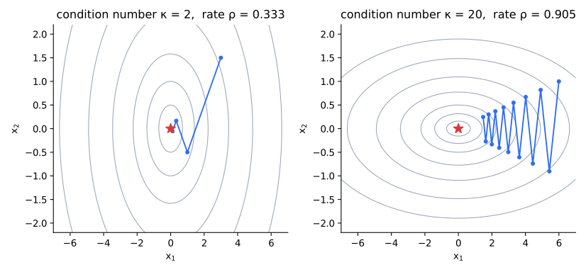
$$k\;\approx\;\frac{\kappa}{2}\,\ln\frac1\varepsilon .$$

The iteration count is linear in the condition number. Figure 1 shows why: along the steep direction the step overshoots and alternates sign, while along the shallow direction it barely moves.

Contours of two quadratics with condition numbers 2 and 20 and the zig-zag path of gradient descent with the optimal fixed step — Figure 1. Gradient descent with the optimal fixed step $2/(\lambda_1+\lambda_d)$, 14 steps, on $f=\tfrac12(x_1^2+\kappa x_2^2)$. Left: $\kappa=2$, $\rho=0.333$. Right: $\kappa=20$, $\rho=0.905$. The red star is the minimiser.

3. Conjugate gradient: $\sqrt\kappa$ instead of $\kappa$

The conjugate gradient method (Hestenes & Stiefel, 1952) solves $A\mathbf x=\mathbf b$ with the same cost per iteration as gradient descent, one product with $A$, but it builds each search direction to be $A$-orthogonal to the previous ones. In exact arithmetic it finishes in at most $d$ steps, and its error obeys the bound (Shewchuk, 1994, eq. 52)

$$\|\mathbf e_k\|_A\le 2\left(\frac{\sqrt\kappa-1}{\sqrt\kappa+1}\right)^{k}\|\mathbf e_0\|_A ,$$

which gives $k\approx\frac{\sqrt\kappa}{2}\ln\frac2\varepsilon$ iterations. The condition number enters through its square root.

4. Least squares is a quadratic, and the Hessian squares the conditioning

For a design matrix $X\in\mathbb R^{n\times d}$ the least-squares loss $\frac1{2n}\|X\mathbf w-\mathbf y\|^2$ is a quadratic with $A=X^\top X/n$ and $\mathbf b=X^\top\mathbf y/n$. The eigenvalues of $X^\top X$ are the squared singular values of $X$, hence

$$\kappa(A)=\kappa(X)^2 .$$

Features with very different scales, or with a large mean next to a small variance, make $\kappa(X)$ large and $\kappa(A)$ its square. Two preprocessing steps address this. Centring each feature makes it orthogonal to the intercept column, because $X_{\cdot j}^\top\mathbf 1=0$; the matrix $A$ then becomes block diagonal, $\mathrm{diag}\bigl(1,\,C\bigr)$, with $C$ the sample covariance matrix of the features. Scaling each feature to unit variance turns $C$ into the correlation matrix, whose diagonal is all ones. If features are close to uncorrelated, $C\approx I$ and $\kappa\approx1$.

5. Implementation

The two solvers in NumPy. The complete script, including both experiments and both figures, is downloadable.

import numpy as np

def a_norm(A, e):
    return float(np.sqrt(e @ (A @ e)))

def gd_iters(A, b, x_star, step, tol=1e-6, cap=300_000):
    """Fixed-step gradient descent from x0=0; stop when ||e_k||_A <= tol * ||e_0||_A."""
    x = np.zeros_like(b)
    e0 = a_norm(A, x - x_star)
    for k in range(1, cap + 1):
        x = x - step * (A @ x - b)
        ratio = a_norm(A, x - x_star) / e0
        if ratio <= tol:
            return k, ratio
    return None, ratio

def cg_iters(A, b, x_star, tol=1e-6, cap=100_000):
    """Conjugate gradient from x0=0 with the same stopping rule."""
    x = np.zeros_like(b); r = b - A @ x; p = r.copy(); rs = r @ r
    e0 = a_norm(A, x - x_star)
    for k in range(1, cap + 1):
        Ap = A @ p
        alpha = rs / (p @ Ap)
        x = x + alpha * p
        r = r - alpha * Ap
        if a_norm(A, x - x_star) <= tol * e0:
            return k
        rs_new = r @ r
        p = r + (rs_new / rs) * p
        rs = rs_new
    return None

Sanity check

On the 2-D quadratic $\mathrm{diag}(1,50)$ with the optimal step, the error norm after 25 steps divided by the initial one is $0.3678304$, identical to $\rho^{25}=(49/51)^{25}$ to the printed digits: for this matrix the rate is attained exactly, not just bounded.

6. Experiment 1: gradient descent vs. conjugate gradient

Setup (synthetic, fully reproducible). For each $\kappa\in\{10,10^2,10^3,10^4\}$, $A=Q\,\mathrm{diag}(\lambda)\,Q^\top$ with $d=100$, a random orthogonal $Q$, and eigenvalues log-spaced from 1 to $\kappa$; $\mathbf b$ is standard normal, $\mathbf x_0=\mathbf 0$, NumPy seed 3. Gradient descent uses the optimal fixed step $2/(\lambda_1+\lambda_d)$. I count iterations until $\|\mathbf e_k\|_A\le10^{-6}\|\mathbf e_0\|_A$ and compare them with the bound, $\lceil\ln(10^{-6})/\ln\rho\rceil$ for gradient descent and $\lceil\ln(10^{-6}/2)/\ln q\rceil$ for conjugate gradient, with $q=(\sqrt\kappa-1)/(\sqrt\kappa+1)$.

κ	GD bound	GD measured	CG bound	CG measured
10	69	60	23	21
100	691	633	73	59
1,000	6,908	6,241	230	131
10,000	69,078	59,014	726	272

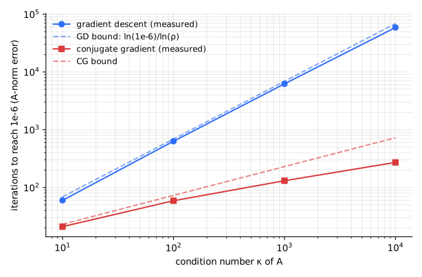
Log-log plot of iterations to reach 1e-6 versus condition number for gradient descent and conjugate gradient, measured and bound — Figure 2. Iterations to reach $10^{-6}$ in the $A$-norm versus condition number (log–log). Output of the script in this article.

Gradient descent scales linearly with $\kappa$. Each factor of 10 in $\kappa$ multiplies the measured count by about 10 (60, 633, 6,241, 59,014) and stays below the bound.
Conjugate gradient scales roughly with $\sqrt\kappa$. From $\kappa=10$ to $10^4$ the measured count grows from 21 to 272, a factor of 13, while $\sqrt\kappa$ grows by a factor of 32; it is below its bound throughout and well below it at large $\kappa$; Shewchuk notes that CG often beats the bound when the eigenvalue distribution is favourable.
At $\kappa=10^4$ the gap is 59,014 against 272 iterations, about 217 times, for the same cost per iteration.

7. Experiment 2: standardising features in a regression

Setup (synthetic, fully reproducible). $n=2000$ “houses” with an intercept and four features: area $\sim\mathcal N(100,30^2)$, number of rooms uniform on $\{1,\dots,6\}$, age $\sim U(0,50)$, distance $\sim\mathcal N(5,2^2)$; target $y=X\mathbf w+\mathcal N(0,5^2)$ with $\mathbf w=(20,\,1.5,\,4,\,-0.3,\,-2)$ (NumPy seed 5). The loss is $\frac1{2n}\|X\mathbf w-\mathbf y\|^2$, $A=X^\top X/n$, start at $\mathbf w=\mathbf 0$, optimal fixed step, same stopping rule, cap of 300,000 iterations. Three versions of the same data: raw, centred, and centred and scaled to unit variance.

Features	κ(A)	GD bound	GD measured	CG measured
raw	3.04×10⁵	2,099,254	not reached in 300,000 (error ratio 0.139)	6
centred	866.0	5,983	5,982	5
centred + unit variance	1.087	5	4	4

Raw features: the eigenvalues of $A$ range from 0.0382 to 11,615, $\kappa=3.04\times10^5$. After 300,000 iterations gradient descent has still only reduced the $A$-norm error to 13.9% of its start; the bound predicts about 2.1 million iterations to reach $10^{-6}$.
Centring alone reduces $\kappa$ by a factor of 350 (to 866), and gradient descent then needs 5,982 iterations, which is within one iteration of the bound.
Centring and scaling gives $\kappa=1.087$: four iterations, because the features here are nearly uncorrelated and $A$ is close to the identity.
Conjugate gradient needs 4–6 iterations in every case. With $d=5$ unknowns, exact arithmetic would finish in at most 5; the 6 on the raw data is consistent with floating-point rounding at $\kappa\approx3\times10^5$.

Limitations. Both experiments are quadratics, where $\kappa$ is constant; for non-quadratic losses the relevant matrix is the local Hessian and it changes along the path. The optimal step uses the exact extreme eigenvalues, which one rarely knows; with a safe step such as $1/\lambda_d$ the rate is $1-1/\kappa$, slower still. The features in Experiment 2 are nearly uncorrelated, so standardising brings $\kappa$ close to 1; strongly correlated features stay ill-conditioned after standardising, because $C$ then has small eigenvalues. There is no regularisation, which would also bound $\lambda_1$ from below. All data are synthetic.

8. Practical takeaways

Centre and scale features before using any gradient-based solver on a linear or generalised linear model. It costs two lines and can change the iteration count by orders of magnitude.
Remember $\kappa(X^\top X)=\kappa(X)^2$: for a direct solution of least squares prefer QR or SVD over the normal equations, as the eight-point article argued for coordinates.
For large sparse or structured quadratic problems, conjugate gradient pays $\sqrt\kappa$ rather than $\kappa$ for one matrix-vector product per iteration.
Look at the condition number (or the ratio of the largest to smallest eigenvalue of the Hessian) when training is slower than expected, before touching the learning rate.
Check correlations after standardising: they set the condition number that remains.

Need a data pipeline, a chatbot agent or a custom AI tool?
I build these as a freelancer. Describe your project in a few sentences and I will reply with questions and a fixed-scope quote.

Ask for a quote See services

References

M. R. Hestenes and E. Stiefel. “Methods of conjugate gradients for solving linear systems.” Journal of Research of the National Bureau of Standards 49(6):409–436, December 1952 (Research Paper 2379). PDF.
J. R. Shewchuk. “An Introduction to the Conjugate Gradient Method Without the Agonizing Pain.” School of Computer Science, Carnegie Mellon University, edition 1¼, August 4, 1994. Author page. (Steepest descent and conjugate gradient convergence in terms of the condition number; the factor-2 bound is Eq. 52.)
S. Boyd and L. Vandenberghe. Convex Optimization. Cambridge University Press, 2004. Book page. (Chapter 9: gradient descent for strongly convex functions.)
R. I. Hartley. “In defense of the eight-point algorithm.” IEEE TPAMI 19(6):580–593, 1997. doi:10.1109/34.601246.

Code: gd_conditioning.py (Python 3.12, NumPy, Matplotlib). All numbers in Sections 5–7 are the output of this script.